The Inertial Properties of the Apollo Lunar Excursion Module (LEM)
How balanced was the LEM (in terms of rotational inertia)?
The CSM/LM Spacecraft Operational Data Book. Volume 3: Mass Properties (Revision 2, 20. August 1969, Manned Spacecraft Center, Houston Texas, USA) on table 3.1-3 on page 3.1-11 (PDF page 61) prints the raw numbers that allows us to see that — despite its irregular appearance — the LEM was balanced very well across its three axes.
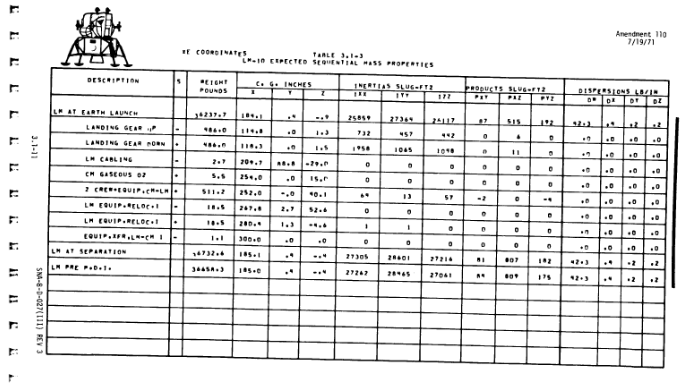
The table is titled “expected sequential mass properties”; the key rows give the numbers for each milestone in the mission. We’re interested in the “LM pre P.D.I.” which is in the last row of the table.
Next to the “weight pounds”, the table features the column “C.G. inches”. Weight and the location of the center of gravity completely specify the translational inertia of the vehicle, which is of no further interest to this blog post.
The columns “inertias slug-ft2” (
This tensor is represented by a symmetric 3x3 matrix. Let’s assemble it from the 6 values given in the book:
The choice of unit — slug-ft² — appears peculiar to my ‘modern’ eye; I mean, slug square feet?? Let’s convert this to SI units using 1 slug = 14.59390 kg, 1 foot = 0.3048 m, 1 pound = 0.45359237 kg:
The off-diagonal elements are also called the products of inertia.
On the top of the table we read that the numbers are in “XE coordinates”; in Figure 2-12 on page 2-13 (PDF page 37) we see that that is the “LM Coordinate System” (with the +X axis out the docking interface, the +Z axis out the windows, and the +Y axis completing the right-handed coordinate system). So, the basis of this matrix is the LM coordinate system.
The fact that the matrix is not purely diagonal tells us that the LEM’s principal inertial axes did not coincide exactly with the LEM’s coordinate system. However, the fact that the diagonal elements are much larger than the off-diagonal elements, and are of roughly the same magnitude, already tells us that the LEM was balanced well.
But, how well was it balanced, exactly? To find that out, we have to know a bit of mathematical mechanics: The inertia matrix becomes diagonal when its base coincides with the principal inertial axes1 (any symmetric matrix can be diagonalized by a change of basis2).
This change of basis means a rotation of the coordinate system; the eigendecomposition of a matrix3 gives4 the following (orthogonal, unit length) base vectors of the new coordinate system, also called the Eigenvectors of the matrix:
Each Eigenvector has an associated Eigenvalue, which can be assembled to yield the diagonal inertia matrix:
Norming this matrix relative to the middle value (the Y axis), we can see even better how well the LEM was balanced:
Roughly speaking, rotating the LEM around its X axis (the axis from its ‘feet’ up to the docking hatch) was around 10% easier than around its other two axes.
Visualization
Now, let’s visualize how much the Eigenvectors are rotated away from the LEM’s coordinate system by inputting the original Inertia Matrix into my Eigenvector Visualizer. As you can see, the angle offsets of the Eigenvectors are quite dramatic: almost 45 degrees away from the X axis! But, in practice this was of no concern because the Eigenvalues were extremely well balanced. This can be illustrated by turning on “Show Poinsot’s Construction” below and seeing that the shape of the red inertial ellipsoid is almost congruent with the blue semitransparent sphere.
Dynamic simulation
The mass of this particular LEM, according to the data sheet shown above, was 36658.3 pounds (16628 kg), with 16 x 440 N of thrust.
With these numbers at hand, and based on my previous implementation of the simulation of Rigid Body rotations with propulsion, it now becomes possible to realistically, dynamically, and even interactively simulate the inertial behavior of the LEM in all its glory.
The 3-dimensional model of the Apollo Lunar Module used in the visualization below was made available by NASA (here and here).
The displayed grid is 100 meters cubed, and the LEM is placed in the middle.
Thrusters
Quad A (left-fwd):Quad B (left-aft):
Quad C (right-aft):
Quad D (right-fwd):
Combinations
L =
| +0.000 |
| +0.000 |
| +0.000 |
| +0.000 |
| +0.000 |
| +0.000 |
| +35717.00 | +0.00 | +0.00 |
| +0.00 | +37853.00 | +0.00 |
| +0.00 | +0.00 | +38675.00 |
Erot = 0.000 J
Etrans = 0.000 J
|L| = 0.000
Footnotes
https://en.wikipedia.org/wiki/Moment_of_inertia#Principal_axes ↩
https://en.wikipedia.org/wiki/Eigendecomposition_of_a_matrix ↩
Using my own interactive Eigenvector and Eigenvalue visualization. Numbers verified using independent online services 1, 2 and 3. ↩